The Physics of Boids

Simulating Boids appears to have become quite a common coding exercise and is well covered, both as great YouTube content and extensively across blogs, so I had not planned to add my own take on it when I started to explore the seemingly simple set of rules that yield complex and organic looking visuals of emergent flocking behaviour. After diving deeper into the topic, however, most sources of information on the topic appear to focus on the classic set of 3 rules, performance optimisations and, if you’re lucky, a list of ‘magic’ coefficients to make it work, which didn’t sit well with me.

In this article I hope to provide a more intuitive framework for the Boids simulation, simplifying the rules and provide a reasonable argument for how rules combine in a more forgiving and intuitive way.

Boids Overview

Rules

Before introducing my own take on the rules and the corresponding physics-based framework, I want to start with the core concepts of the Boids simulation introduced in 1987 by Craig Reynolds. The original paper proposes that in order to simulate organic and complex flocking behaviour, similar to what you may see with certain kinds of birds and fish, only a simple set of three rules are required that each participant, or boid, follows:

1. Centring - Stay close to centre of the group of every other you can see around you
2. Matching - Match your velocity to those you see around you
3. Avoiding - Avoid getting too close to those you see around you

Although sufficient to achieve a realistic looking flocking behaviour, in almost all practical cases certain boundary conditions exists, e.g., when leaving one side of the space the simulation runs in a boid is ‘warped’ to the opposite side, but more often boids are diverted away from the simulation boundaries in a similar way they might avoid other objects, creating an optional but often implemented 4th rule:

1. Dodging - Dodge boundaries and objects to avoid a collision

These rules are then combined in a weighted manner, with weights generally found by trial-and-error until the result is visually pleasing. The process of finding these weights can be challenging, because three forces need to be balanced at the same time.

Parameters

Every Boids simulation takes place inside a certain simulation volume and / or at a certain scale, which will contextualise aspects such as the size, position, velocity, etc. of each boid. For example, in the simulation I wrote, each boid was displayed with a bird-like model, having a bounding box of around 10x10x10 units inside Unity. Which can be used to start to set the main set of variables that control the main visual aspects of a Boids Simulation:

• The range within a boid will try to avoid others: $r_a = 10$, the size of the Boid’s ‘span’.
• The range within a boid can see others: $r_v = 30$, about 3 bird spans, or around 25 birds separated by a distance of ~10 within a sphere.
• (optional) The fraction of the field each boid can see: $\theta_v = 0.8$, meaning that in a 2D simulation the opening angle is $0.8 \times 2\pi$ rad and in 3D $0.8 \times 4\pi$ sr, to simulate a boid’s inability to look directly behind them.

I ended up simulating a volume of $500^3$ units, with ~250 boids in it, giving each about 50 cubic ‘spans’ of free range in each direction on average. I found most values of 50 or higher to work well in 3 dimensions for the above paramenters. Smaller values, and thus more densely packed boids, will work, but tend to converge to a single large flock dominating the volume.

Schematic Overview

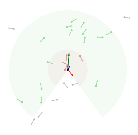
To explore the impact of each force, I’ll be using an abstract 2D representation for one boid as shown below, with $r_a$ in red, $r_a$ in green, each boid’s location as a dot and its velocity vector indicated by an arrow. And although in practice, all boids are observing each other and have similar forces applied to them, focusing on what one of them ‘sees’ makes things easier to illustrate. The main boid under consideration is coloured in black, whereas all others are coloured according to the ‘zone’ they are in:

Physics Based Framework

Centring

Most simulations will have one force to nudge each boid to the centre of mass and another to nudge the direction of travel towards the average direction of their visible neighbours, however, it felt more natural to me to combine these two rules into one and nudge each boid toward where the centre of mass will be in the future, given its current position and velocity. It is in essence almost the same thing, but the relative importance between the position and velocity of the group has now a more intuitive meaning. I also found it more natural to assume that animals that show flocking behaviour would instinctively aim for where the others will be in the future instead of where they are now, similar to how a person would throw or kick a ball ahead of another player in sports to account for the ball’s travel time, instead of correcting for both aspects separately.

To know what amount of acceleration is needed to move a given boid (i) to the Centre of Mass (CM) of the other boids it can see, I assume a simple extrapolation of the current location of the CM and the boid itself, with $a_i$ to solve for:

$$\vec{x}_i + \vec{v}_i \Delta t + \frac12 \vec{a}_i \Delta t^2 = \vec{x}_{CM} + \vec{v}_{CM} \Delta t \tag{1}$$

$$\vec{a}_i = \frac{2}{\Delta t^2} \left[ (\vec{x}_{CM} - \vec{x}_i) + \Delta t(\vec{v}_{CM} - \vec{v}_i) \right] \tag{2}$$

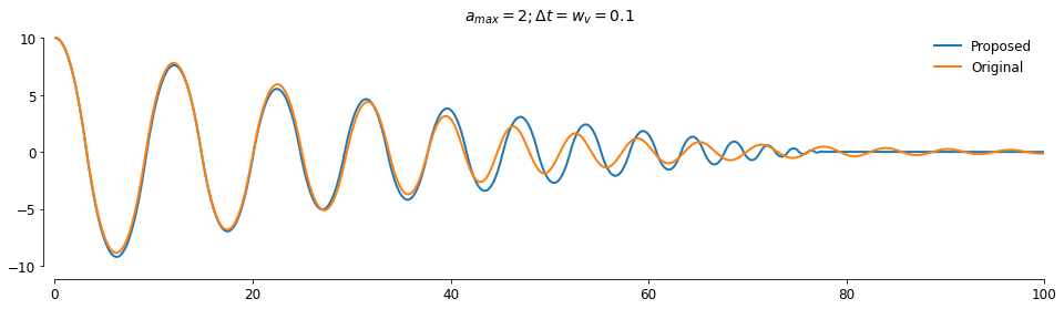
The equation for the acceleration (or force for a mass of 1) that will nudge a boid towards the future location of the centre of mass (CM) is very similar to have force for the location and average direction separately, with the velocity component weighted by a factor of $w_v = \Delta t$. Below, I’ve plotted the subtle difference in behaviour that achieved by coupling the two parts (Proposed column) vs. not (Original column). The scenario plotted here is a case where 1 boid starts out at $\vec{x}_0 = (0, 10)^T$ traveling with a velocity $\vec{v}_0 = (1, 0)^T$ and the CM starts out at $\vec{x}_0 = (0, 0)^T$ traveling with a velocity $\vec{v}_0 = (1, 0)^T$. The first thing that jumps out is that in both cases the boid will undulate around the CM moving to the right, due to overcorrection until it ultimately aligns with the CM. The main difference though, is that with the original approach a more asymptotic approach towards the moving CM can be seen, whereas with the proposed version the approach is more linear and stabilises a bit earlier.

Note that I’ve used here a cap on the maximum acceleration that can be achieved, because the proposed version will otherwise asymptote almost immediately since the applied acceleration is almost exactly what is required to arrive at the CM at $t + \Delta t$. Additionally, no animal can accelerate instantaneously to arbitrary degrees, so for the simulation I’ve applied a maximum acceleration based on what a reasonable turning radius would be for the boid given the maximum allowed velocity in the simulation which is mostly determined by what looks visually pleasing. For my simulation, that ended up being $v_{max} \in [2, 5]$ and a minimum turning radius $r_{min} \in [15, 25]$ or about 1.5 to 2.5 bird ‘spans’, which yields a maximum acceleration of $a_{max} = v^2_{max} / r_{min} \in [0.16, 1.67]$. For illustration purposes I’ve used $a_{max} = 2$ and much larger values further down to emphasise the impact on the boids’ behaviour.

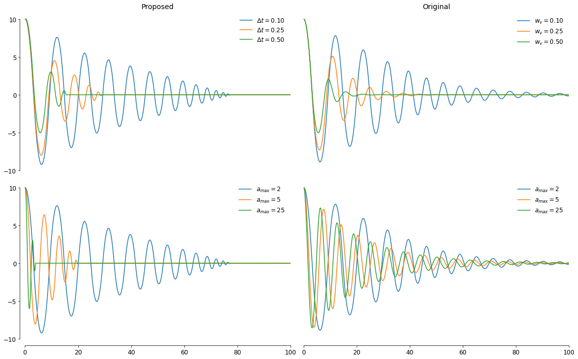
To illustrate the impact of and get a feel for changing the $\Delta t$ or equivalent $w_t$ in the original approach, I’ve plotted it for various values, and as expected, with larger values, it asymptotes more quickly, because it dampens the amount of over-correcting the boid does in order to catch up. I also added two plots to show the impact of lifting the limit on the amount of acceleration a boid can achieve, and as expected, under the original approach, not much changes but for the proposed version it also asymptotes more quickly. This allows for a nice balance between how quickly a boid can turn and how quickly it matches the velocity of the CM. My interpretation of this setup is that animals that can update their bearings more quickly - and thus have a lower $\Delta t$ - tend to emphasise co-location over velocity matching, e.g., birds, whereas animals that may be slower to process visual cues, e.g., sardines, tend to emphasise velocity matching much more.

Avoiding

For avoiding other boids, I found a variety in treatments in online available sources but most fell into broadly two categories: Proportional to the distance or the reciprocal distance, and practically all are adding the forces from all nearby boids to avoid together, making the net force depend on the number of boids that are ‘too close for comfort’. Especially that last part didn’t sit well with me, because an animal in a flock would not start moving twice as fast just because there are two others nearby vs. only one at approximately the same location. In the end I landed on a similar approach as I used for the centring force, by calculating a weighted Centre of Mass to move away from. The weighting is based on how close the others each are $r_a$, assuming that the net impact of a boid at the boundary should be zero and proportionally higher as it is nearer by.

Solving a similar equation as eq. 1, where the ideal amount of acceleration is based on what it would take to move away from this weighted CM, similar to eq. 2:

$$\vec{a_i} = \frac{2}{\Delta t^2} \vec{x'}_{CM} \tag{3}$$

where the $\vec{x'}_{CM}$ is the future location of the weighted CM:

$$\vec{x'}_{CM} = \sum^{r_i \leq r_a}_{i \neq j} (r_a - r_i) \left( \frac{\vec{x}_i + \vec{v}_i \Delta t}{r_i} \right) \tag{4}$$

where $r_i = ||\vec{x}_i + \vec{v}_i \Delta t|| + \epsilon$. The added $\epsilon$ is to avoid division by zero errors from any, albeit unlikely, zero vectors.

Combining Forces

With eq. 2 and 3, the net applied acceleration can be calculated for each boid, capping the magnitude at a given $a_{max}$. Below, I’ve plotted the calculated acceleration vectors for Centring (green) and Avoiding (red), each pointing at its respective (weighted) CM to move towards, or away from respectively. The capped combined vector is shown in blue, indicating the actual direction the boid would be moving towards.

With the two accelerations in hand, it is also possible to re-balance their importance for the boids, mixing them with $\theta$ and $1 - \theta$ weights. From experimentation with various values in my simulation, a mix of 1-2% of the Centring acceleration and 99-98% of the Avoiding acceleration gives a pleasing visual result. This is also what I would have expected, that avoiding neighbours - and avoid injury presumably - is a higher priority effectively than keeping up. Some of the balancing is also a result of the radius of each region, with the Centring vector potentially as large as $r_v$ and the Avoiding vector only ever as large as $r_a$, which in my simulation are a ratio 3:1 in size respectively. There is probably an opportunity here to further normalise the system of equations by these ranges and account for the likelihood of seeing another boid in each region in the final weights, and I may get back to that at a future time.

Extra Rule: Object Avoidance

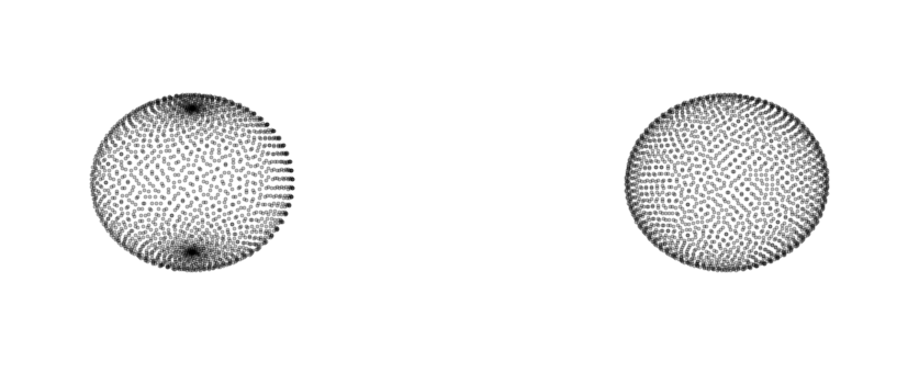
Object avoidance is an important aspect of any flocking / boids simulation, if anything to keep all boids inside a certain volume for visualisation purposes. The original paper describes a process to find a direction that deviates the least from the current direction of travel and is unobstructed. To find this free direction to move towards, I used a common ray casting technique where you start in the ‘forward’ direction of the boid and then iteratively increase the pitch by a small amount, and the roll around the travel direction by an amount that minimises repetition. A common value for the latter is the (inverse) golden ratio as the most irrational number. In spherical coordinates: $\Delta \theta = \arccos(1/n)$ and $\Delta \phi = \pi \left( \sqrt{5} - 1 \right)$. The $\arccos$ for the pitch is important to correct for the bunching at the poles you would get with a uniform distribution, i.e., $\Delta \theta = 1/n$:

The acceleration needed to avoid a collision then becomes:

$$\vec{a}_i = \left( ||\vec{v}_i||\hat{v}_{free} - \vec{v}_i \right) / \Delta t \tag{5}$$

which can then be mixed in with the other two forces. For experimentation, prioritising the obstacle avoiding above all else gives the best results, and a mixture of 50% obstacle avoidance 49% boid avoidance and 1% centring gave me robust flocking behaviours in a 3D simulation. Below is a video capture of the simulation, but the quality is quite poor due to the challenge with video compression of lots of small moving objects while trying to keep the file relatively small:

Note that for the simulation shown in the video I did not add a dominant initial direction to the boids, counter what appears to be common practice, to emphasise the interaction of the forces when the global CM is not moving much.

Conclusion

Based on these explorations, I feel that a system of equations rooted in a more physical approach has value for Boids simulations, making the choice of parameters that govern the visual effect less opaque. That said, I’ve not seen anything that leads me to believe either approach produces more pleasing visuals than the other. Hopefully this approach can be helpful to others that look to explore creating a Boids simulation in the future and, if anything, shorten the amount of time needed to find the right balance of influences on each boid to achieve the desired visual effect.

---

This page has been converted from a Jupyter Notebook with most of the code removed for an improved reading experience, however, if you are interested in reading through the code behind the plots and / or playing around with the original notebook, it can be downloaded here. The simulation I created in Unity for this exploration didn’t feel sufficiently interesting to share as a standalone build, but if you are interested in using the source code for your own project, feel free to reach out.