Exploring the Lennard-Jones Potential

This article is the start in a series of explorations into emergent properties and behaviours stemming from rules that appear to be extremely simple at face value but lead to complex results, nevertheless. And to start, I wanted to dive into a topic that has interested me for a while now but hadn’t really taken the time to explore before: Using the GPU’s compute capacity, and what better topic to start with than an N-body problem.

My main language of choice for most projects is Python, but for one of them I had used Unity and realised it would be simpler to use the GPU for the mathematics and the Unity engine to display the motions of the N-bodies in 3D, and that it would be a lot more work to achieve the same Python. The result is an interactive simulator of the Lennard-Jones Potential, which can be found on itch.io, but it took a few steps to get there, which I’ll share here as well.

Before diving into the details, I want to share these two sources I used as a jumping off point to get started with doing N-body calculations using Compute Shaders and showing the results using Procedural Instancing in Unity: catlikecoding.com and tzaeru.com. Both were immensely helpful for me to get started and do a much better job at conveying the code pieces than I could here to anyone interested in exploring similar topics.

Introduction

When looking at N-body simulations the traditionally obvious place to start is with gravity and simulating galaxies or solar systems, but I found those not to be as interesting, partially because of what I was able to produce in terms of scale and complexity was quite limited, and the emergent behaviour was more intuitive. My mind then went back to other interesting interaction models I learned about in school at some point, and I remembered learning about the attractive-repulsive potential that is often associated with van der Waals forces and dove into the rabbit hole of the Lennard-Jones Potential. The potential itself is mathematically quite simple, which describes the potential energy of a particle with respect to another particle depending on the distance separating them:

$$V_{LJ}(r) = 4\varepsilon \left[ \left( \frac{\sigma}{r} \right)^{12} - \left( \frac{\sigma}{r} \right)^6 \right]$$

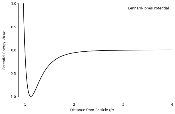
The potential has an attractive and repulsive part, which is governed by the $-r^{-6}$ and the $r^{12}$ terms respectively:

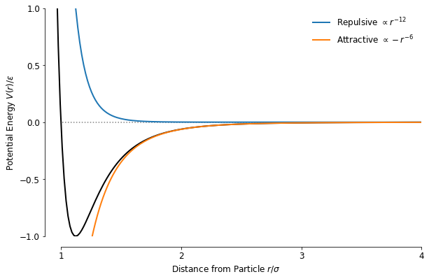
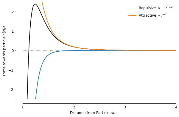
The potential itself will be useful again later, but I found it much easier to reason about the attractive-repulsive behaviour when looking at the force, which is the derivative of the potential. The expression for the force is also more helpful for simulating the particle-particle interactions later:

$$F_{LJ}(r) = \frac{dV_{LJ}(r)}{dr} = 24 \frac{\varepsilon}{\sigma} \left[ \left( \frac{\sigma}{r} \right)^7 - 2 \left( \frac{\sigma}{r} \right)^{13} \right]$$

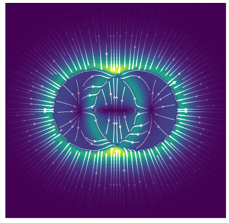
One aspect that I didn’t touch on yet is the radial symmetry of the function, which I showed only in its traditional form in 1D so far, and to get a bit more intuition for how the forces play out between particles, I plotted the force vector fields around 3 roughly equidistant particles in a 2D plane, with their midpoints separated by around $3\sigma$ from each other.

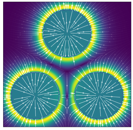
It’s interesting to see the thin rings of stability where both repulsion and attraction are in balance around each particle’s “horizon of repulsion” - the edge of each flat circle - corresponding to the minimum potential energy at that distance and where thus the net force is zero. Similarly, the thick bright yellow/green ring shows where the attractive force is the highest. The distance particles need to be to be stably bound turned out to be much closer than I would have expected based on the above picture, because naively, looking at the plot I would have thought that the closest each particle could get to each other would be when those horizons touch, but that’s not the case. What happens is that each particle’s mass is assumed to be only located at its centre, so it is the distance between the centres of each that matters.

The point where the total potential energy is minimized between two particles is at a distance of $2^{1/6}\sigma$ between their centres, which gives the following corresponding force field, different from what I had initially expected.

Potential and Kinetic Energy

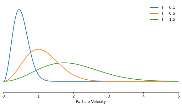
To make the group of particles that I want to simulate resemble something more realistic, the matter will need to have a couple of macro descriptions like temperature and density to work with. Luckily, both of those have a well-established relationship with the micro parameters each of the particles will have in the simulation, with the density determining the average distance between the particles, and the temperature the average speed. The exact relationship between the speed of the particles and the temperature is described by the Maxwell-Boltzmann distribution, which arises from particles transferring part of their momentum in collisions to other particles over time.

Using the Maxwell-Boltzmann distribution, given a certain temperature, it predicts a distribution of speeds across the group of particles, with the average speed proportional to the square root of the temperature:

$$f_{v} \propto \frac{v^2}{T^{3/2}} e^{-\frac{v^2}{T}},$$

$$\mu_v \propto \sqrt{T}.$$

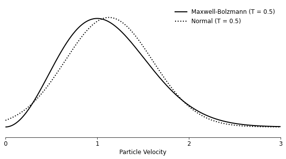
The distribution has a typical slightly skewed shape, because speeds cannot be zero:

Having the speeds to work with for each particle, I can now calculate the total energy of a particle-particle system with a certain velocity and distance:

$$E = E_p + E_k,$$

where the kinetic energy $E_k = \frac12 m v^2$ and the potential energy $E_p$ is governed by the JL potential, and each are mainly determined by the temperature and density respectively.

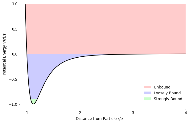
The total energy is helpful to use as an indicator of how a set of particles will behave. For example, if the total is close to -1 for a given particle-particle set then they are located and will generally stay inside each other’s stable zone, without having much velocity themselves and are unlikely to decouple - unless they get knocked loose by a very fast-moving passer-by. With increasing kinetic energy, and thus speed, the pair becomes more easily knocked away from each other by a third particle, and when the net energy is > 0, the pair is unable to bind at all because there is enough kinetic energy to overcome the attractive part of the potential energy.

This diagram shows each ‘zone’, with the division between strongly and loosely bound being quite arbitrary. I used the same colour scheme in the simulation to colour particles depending on the strongest bond they had formed to make it easier to spot changes between the approximate states of matter.

Then taking one more step to use the particle density inside a system as a guide for how far particles will be from each other on average, I was finally able to begin to make sense of the phase diagram and the different states of matter I may see in the simulations later on (as predicted by the diagram I found on Wikipedia):

• Solid (x2): The solid states are located in the region where the density is very high, basically as compact as it can get, and the particles have no place to go and will form a solid almost irrespective of the temperature and thus kinetic energy. What isn’t clear to me is why, with more kinetic energy, the system would go from an HCP (Hexagonal Close Packed) to an FCC (Face Centre Cubic) structure, since they both pack the space equally well. I did observe both states in the simulation at some points but wasn’t able to observe a clear transition.
• Solid & Gas: The solid & gas state is located in the lower regions of density and temperature, where particles are spread out enough to move around, but the kinetic energy is also low, so when particles do meet, they bond strongly with not enough kinetic energy to escape but will wander around alone in the empty space between clusters of particles in the meantime.
• Liquid & Gas: When the temperature increases, the same would happen as in the solid & gas state, but the bonded particles have enough energy to kind of meander amongst each other in clusters bound a bit more loosely as a liquid would. Similar to he solid & gas state, the matter clusters into droplets and free particles meander between those in the meantime.
• Gas or Liquid: When the density goes either up or down from the liquid & gas state, the clusters of particles that are loosely bound will likely becomes one big super cluster, i.e., a liquid, or be so spread out from each other that they practically almost never meet.
• Supercritical: Increasing the temperatures beyond the liquid & gas state, particles are now moving too fast to bond meaningfully, but due to collisions some will be slow enough - see the breadth of the velocity distribution at higher temperatures - to loosely bond for a bit before getting knocked loose again and form a state that is both a gas and a liquid at the same time, which is different from the liquid and gas state where each state could be overserved independently instead of mixed.
• Solid & Liquid: The solid & liquid boundary, appears to me as the phase where the density is becoming high enough for collisions to become very likely, with some particles too tightly packed to move around each other, i.e., solid, but other areas with a bit more wiggle room and tumble about each other like a liquid.

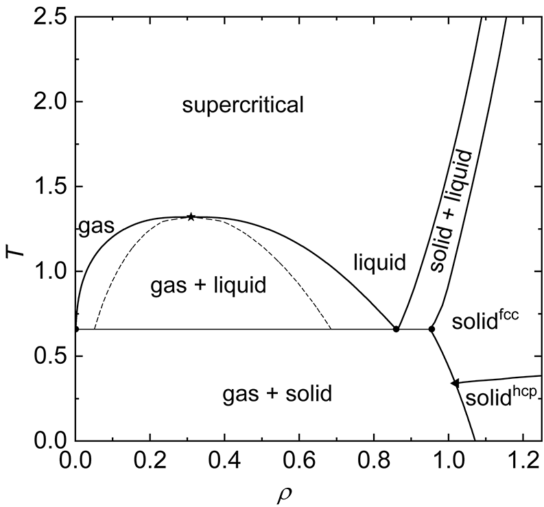
Source: Wikipedia with simplification of axes units mine

Simulation

For the simulation, the forces between each particle-particle pair are used to update their position accordingly in small time steps, which is effectively solving a system of differential equations that describe the equations of Newtonian motion numerically. To keep things as simple as possible, the mass of all particles and $\varepsilon$ were set to 1. The differential equation to solve for each particle-particle combination becomes then:

$$\frac{d^2\vec{x}}{dt^2} = \vec{a}(t) = 24 \frac{\hat{r}}{\sigma} \left[ \left( \frac{\sigma}{||\vec{r}||} \right)^7 - 2 \left( \frac{\sigma}{||\vec{r}||} \right)^{13} \right],$$

which can be solved numerically given an initial speed $\vec{v}_0$ and location $\vec{x}_0$ for each particle.

The challenge when integrating this equation numerically is that not every approach is made equal, and I ended up using one that is typical for this type of problem because of its energy preserving qualities: The Velocity Verlet method, also known as the Leapfrog method. The steps for each timestep are as follows:

1. Calculate the new locations: $\vec{x}(t + \Delta t) = \vec{x}(t) + \vec{v}(t)\Delta t + \frac12\vec{a}(t)\Delta t^2$
2. Calculate the new acceleration based on the new location using the force / acceleration equation at $t + \Delta t$
3. Calculate the new velocities from the average of the old and new acceleration: $\vec{v}(t + \Delta t) = \vec{v}(t) + \frac12(\vec{a}(t) + \vec{a}(t + \Delta t))\Delta t$

In Python-like pseudo code the total integration step would look as follows:

# Each position is a 3D vector
positions[i] += velocities[i] * timeStep + 0.5 * accelerations[i] * timeStep ** 2

for j in range(len(particles)):
    if i == j:
        continue

    direction = positions[j] - positions[i]
    r = np.linalg.norm(direction)

    vec_a += 24 / sigma * ((sigma / r) ** 7 - 2 * (sigma / r) ** 13) * (direction / r)

velocities[i] += 0.5 * (accelerations[i] + vec_a) * timeStep
accelerations[i] = vec_a

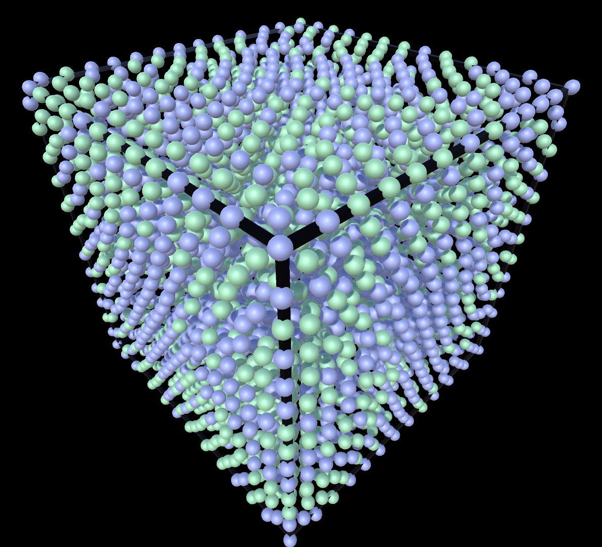
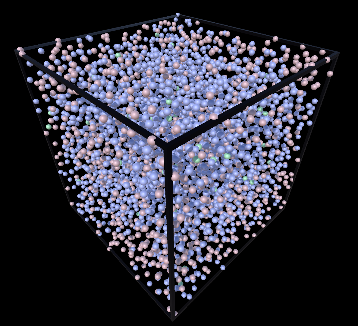
As initial conditions I chose to place all particles inside a 10x10x10 3D ‘box’, with the number of particles fixed to make allocating memory and instructions to the GPU more straightforward. For the images that are following I ended up using a total of $16^3=4096$ particles which was a trade-off between resolution and simulation speed. To keep the simulation run smoothly and make enough in-simulation time pass each second, I needed to simulate roughly 1000 timesteps per second which breaks down into around 50 FPS and 20 simulation steps per frame.

The consequence of that design choice was that $\sigma$ is determined solely by the density, given a fixed box size and number of particles, with a densely packed box, in the solid-state phase, looking as follows:

For the velocities, I chose to draw speeds randomly from a normal distribution with the mean and variance equal to those of the expected Maxwell-Boltzmann distribution the system is expected to asymptote to. Looking at both overlapping, it felt like a sufficiently accurate starting point, even though the mode of each distribution doesn’t line up neatly with the other. I explored the alternative of using the mode of the Maxwell-Boltzmann distribution as the mean of the normal distribution, but that resulted in too few particles with starting temperatures that correspond to the long tail of what we expect and too many with a starting speed close to zero.

Two aspects of simulating this system that arose in the process were:

1. Decreasing potential energy gets converted into kinetic energy, resulting in an increased temperature above the starting point as the system settles into the lower potential energies.
2. Randomly placing particles in a box has a chance of two overlapping sufficiently that their repulsive forces becoming explosively large.

Each was solved for in a somewhat hacky way:

1. A temperature stabilising mechanism was added where the kinetic energy of all particles was reduced or increased in small steps if the system temperature deviated too much from the set temperature. From reading other articles, similar methods have been used for these types of systems.
2. The simulation runs for a few thousand iterations where it doesn’t update the velocities but only the positions to ease the particles away from each other in a more natural arrangement before starting the simulation in earnest.

The result of all this work is a series of interesting emergent phenomena that show a pretty good correspondence between the expected phase changes and what can be seen in the simulation:

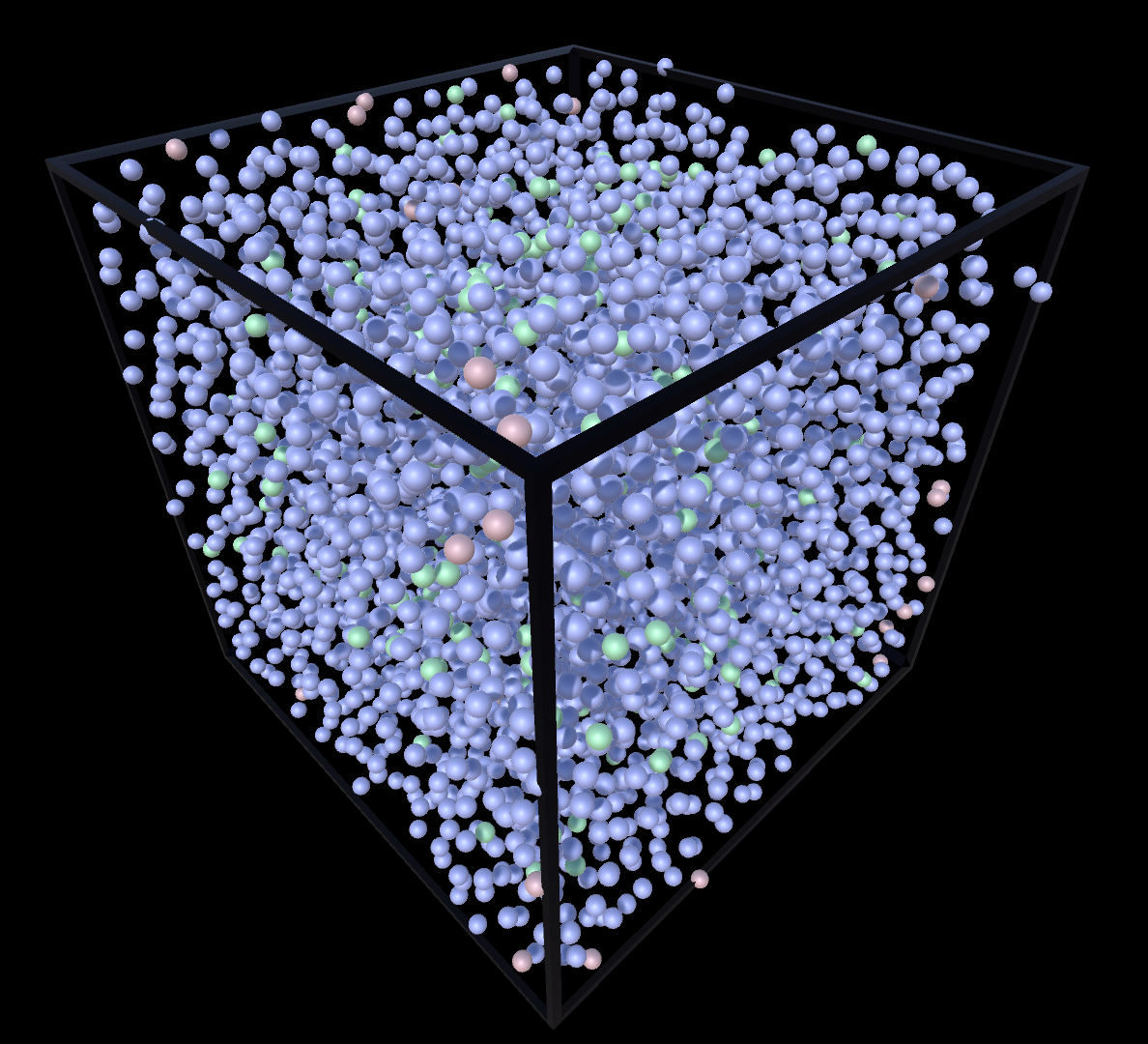
Liquid

Gas

Supercritial

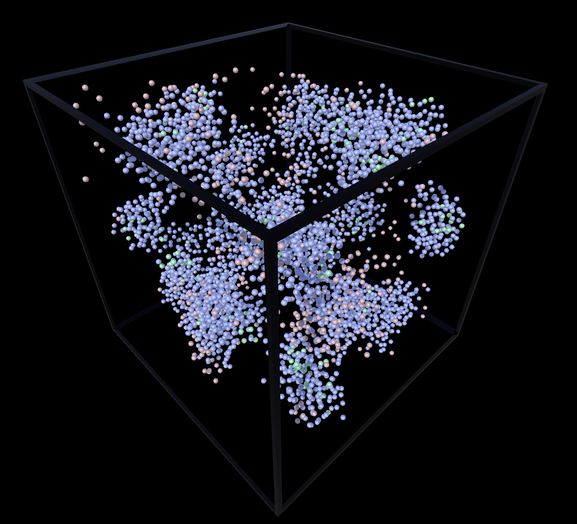
Liquid & Gas

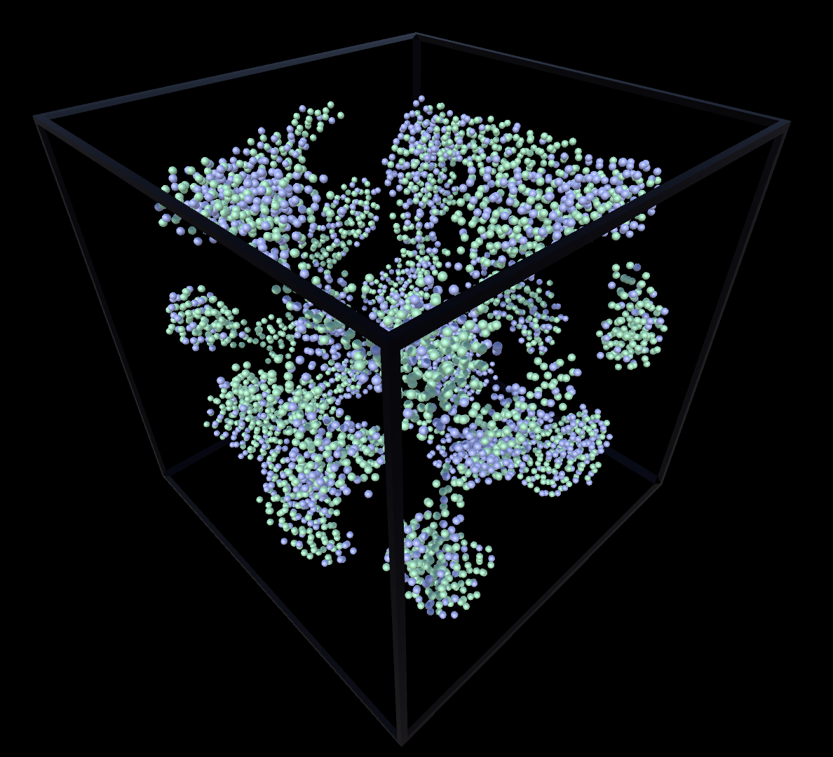
Solid & Gas

Conclusion

I really loved exploring how a simple set-and-forget simulation of 1 simple interaction rule already demonstrated such a rich emergent behaviour and resulted in different states of matter with small changes in the starting density and/or temperature.

This page has been converted from a Jupyter Notebook with most of the code removed for an improved reading experience, however, if you are interested in reading through the code behind the plots and / or playing around with the original notebook, it can be downloaded here. The simulator this exploration resulted in can be downloaded here, and because there is always a non-zero chance that I made some mistakes along the way, and if you spot any, please let me know.