1v3D

Inspired by an online puzzle I had been working on, I was curious to explore the topic of planetary alignment a bit more. The initial premise set out by the puzzel was: Let’s look at times when a set of three planets are colinear with each other when looking ‘top-down’ at the system and assuming they are all moving in the same 2D plane.

Toy Model

To begin, I started with a basic toy model, where planets and their distance to the central star are not necessarily realistic and are purely circular in motion. To be more precise, the planets’ motion is dictated by the following equations:

$$\theta(t) = 2\pi \, t\, /\, k,$$

$$\vec{x}_k(t) = k \begin{pmatrix} \cos \theta(t) \\ \sin \theta(t) \end{pmatrix},$$

with $k$ as both the period and distance to the central star.

def planet(times: np.array, k: int=1) -> np.array:
    theta = 2 * np.pi * times / k
    return k * np.vstack([np.cos(theta), np.sin(theta)]).T

Taking the values provided in the puzzle, $k \in \{3,4,5\}$ and thus the orbital periods relate to each other in ratios of 3 : 4 : 5. This means that after 1 orbit of the planet $x_5$ the other two planets ($x_3$ and $x_4$) will have orbited 5/3 and 5/4 times respectively, and the earliest time all three planets will have made a whole number of whole rations and the system is back to where it started will be after 3 x 4 rotations of planet $x_5$. At that point, all planets will have made 20 : 15: 12 rotations respectively.

Since every orbit of $x_5$ takes 5 time, the system will reset after 60 time has elapsed.

N = 1_000  # samples / yr
T = 60  # years

t345 = np.linspace(0, T, int(N * T) + 1)
p3 = planet(t345, k=3)
p4 = planet(t345, k=4)
p5 = planet(t345, k=5)

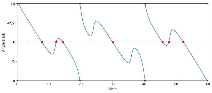
To know if the three planets are colinear there are many possible approaches, but the one I settled on, because I found is easiest to reason about, is to look at the ‘middle’ planet, i.e., $x_4$, calculate the vectors pointing from it to $x_3$ and to $x_5$, and use the inner product to determine the angle the two vectors make. If the angle is either 0 or ±π the planets are colinear:

$$\vec{v}_{34}(t) = \vec{x}_3(t) - \vec{x}_4(t)$$

$$\vec{v}_{54}(t) = \vec{x}_5(t) - \vec{x}_4(t)$$

And because in general

$$\vec{p} \cdot \vec{q}=\left| \vec{p} \right| \left| \vec{q} \right| \cos\theta$$

the angle can be calculated using

$$\theta_{345}(t) = \arccos \frac{\vec{v}_{34}(t) \cdot \vec{v}_{54}(t)}{\left| \vec{v}_{34}(t) \right| \left|\vec{v}_{54}(t) \right|}$$

Unfortunately, when using this method, some information on the relative order of the planets in the alignment is lost because an angle between $v_{34}$ and $v_{54}$ looks the same when their relative ‘order’ is swapped, so I multiplied the angle by the sign of the cross product between the two vectors as additional information:

$${\rm sign}\,(\vec{v}_{34}(t) \times \vec{v}_{54}(t))$$

v34 = p3 - p4
v54 = p5 - p4

d345 = (v34 * v54).sum(axis=1)
n34 = np.linalg.norm(v34, axis=1)
n54 = np.linalg.norm(v54, axis=1)

s345 = np.sign(np.cross(v34, v54))

th345 = s345 * np.arccos(d345 / (n34 * n54))

Here is a animated view of the orbits and the angle they make over time. When animating the planets’ motion and the angle they make together, some interesting phenomena become apparent. For example, the small swings around zero are happening when the two outer planets are straddling the inner orbit, allowing the inner planet to ‘catch up’ and complete the alignment. In that same vein, on two occasions it amounts to a few ‘near misses’. Separately, a jump between ±π appears to happen whenever all three are on the same ‘side’ of the system and form a line ‘in-order’ instead of the ‘out of order’ one when the inner planet sits in the middle.

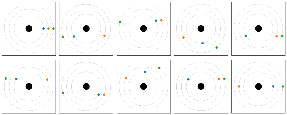
Focussing on only the alignments, there are 10 for each period of 60 time.

Going through the 10 alignments in chronological order, here they are from top-left to top-right and continuing from bottom-right to bottom-left to highlight the circular nature of them.

Earth - Venus - Mercury

After looking at the simplified toy model with integer orbital periods, I was curious to see how this plays out for a slightly more realistic model, albeit still an approximation of course. To start, I assumed that the planetary motions are following by Keppler’s equation for orbits and focussed on our solar system’s three inner most planets only.

The equation of motion I used here is: $$\theta(t) = 2\pi \, t\, /\, T_0,$$

$$\vec{x}(t) = a \frac{1-\epsilon^2}{1 + \epsilon \, \cos \theta(t)} \begin{pmatrix} \cos \theta(t) \\ \sin \theta(t) \end{pmatrix},$$

with $T_0$ the orbit period (in Earth years), $\epsilon$ the eccentricity of the orbit, and $a$ the length of the semi-major axis (in AUs).

To keep it all simple, I made no additional improvements in realism for each orbit, e.g., by correcting for relative rotation, phase, inclination, or otherwise.

def planet_v2(times: np.array, sm_axis: float=1, period: float=1, eccentricity: float=0):
    theta = 2 * np.pi * times / period
    radius = sm_axis * (1 - eccentricity ** 2) / (1 + eccentricity * np.cos(theta))
    return (radius * np.vstack([np.cos(theta), np.sin(theta)])).T

MER = dict(sm_axis=0.387098, period=0.240846, eccentricity=0.205630)
VEN = dict(sm_axis=0.723332, period=0.615198, eccentricity=0.006772)
EAR = dict(sm_axis=1, period=1, eccentricity=0.0167086)

Unlike the orbital periods used in the toy model, the ones for the three actual planets aren’t neat integers or clean ratios of each other, making it hard to know after how much time the system will repeat itself:

• Mercury: 0.240846 year
• Venus: 0.615198 year
• Earth: 1 year

In reality, however, I would not expect an exact return to the starting state to ever occur, e.g., due to the drifting of orbits under the influence of gravitational disturbance, but for this use case a rational approximation would be helpful to get a sense of what time horizon to simulate the orbits for. And it looks like even something like ~1/4 year for Mercury and ~3/5 year for Venus would be reasonable starting approximations, giving ratios of rotations that are 12 : 5 : 3 for Mercury, Venus, and Earth respectively.

That said, using continued fractions a better approximation can be made and maybe provide additional useful approximations.

# Determine the continued fraction of a float
def continued_fraction(val: float, max_depth: int=8) -> list:
    ret = []
    depth = 0

    while val and depth < max_depth:
        v = int(val)
        val = 1 / (val - v) if val - v > 1e-6 else 0
        ret.append(v)
        depth += 1

    return ret

For the periodicity, I mainly care about the ratio of rotations, so approximating the reciprocal of each orbit period directly is easiest.

• Mercury’s rotations / year can be approximated with the continued fraction [4; 6, 1, 1, 2, 1, 2, 1]
• Venus’s rotations / year can be approximated with the continued fraction [1; 1, 1, 1, 2, 31, 3, 10]

# Given a (truncated) continued fraction, determine the rational number a/b 
def approximation_from_cf(cf: list) -> tuple:
    a, b = cf[-1], 1
    for i in cf[-2::-1]:
        a, b = b, a
        a += i * b
    return a, b

Taking the approximations from increasingly adding the number of terms used from each continued fraction, some useful ones jump out:

• Mercury’s rotations / year can be rationally approximated by 4/1 (as initially observed), 25/6, and 54/13
• Venus’s rotations / year can be rationally approximated by 5/3 (as initially observed), 13/8, and 408/251

Taking 25/6 for Mercury and 13/8 for Venus, each <1% off from the original number when expanded into a decimal representation, the rotation of each planet has a ratio of 100 : 39 : 24 to each other, which is quite close to the original (naive) assumed one of 96 : 40: 24 (12 : 5 : 3), with mainly the biggest difference for Mercury. For now, I’ll stick with approximately 3 years as the period to focus on as ‘good enough’, and accept that it doesn’t contain a close to whole set of periods especially for Mercury.

N = 1_000  # samples / year
T = 3.25  # years (3 years + safety margin)

t_evm = np.linspace(0, T, int(T * N) + 1)
p_m = planet_v2(t_evm, **MER)
p_v = planet_v2(t_evm, **VEN)
p_e = planet_v2(t_evm, **EAR)

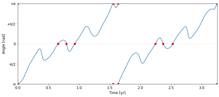
An animated view shows that the features in the more realistic setup appear to be very similar to the one form the toy model, however, due to Mercury’s shorter orbital period, it provides more opportunities for alignment while Venus and Earth straddle its orbit, which incidentally is also a bit smaller relatively as the one used in the toy model, further aiding the chance for alignment.

Focussing on only the alignments again, it’s interesting that we end up with 9-10 alignments in a 3.25 year period.

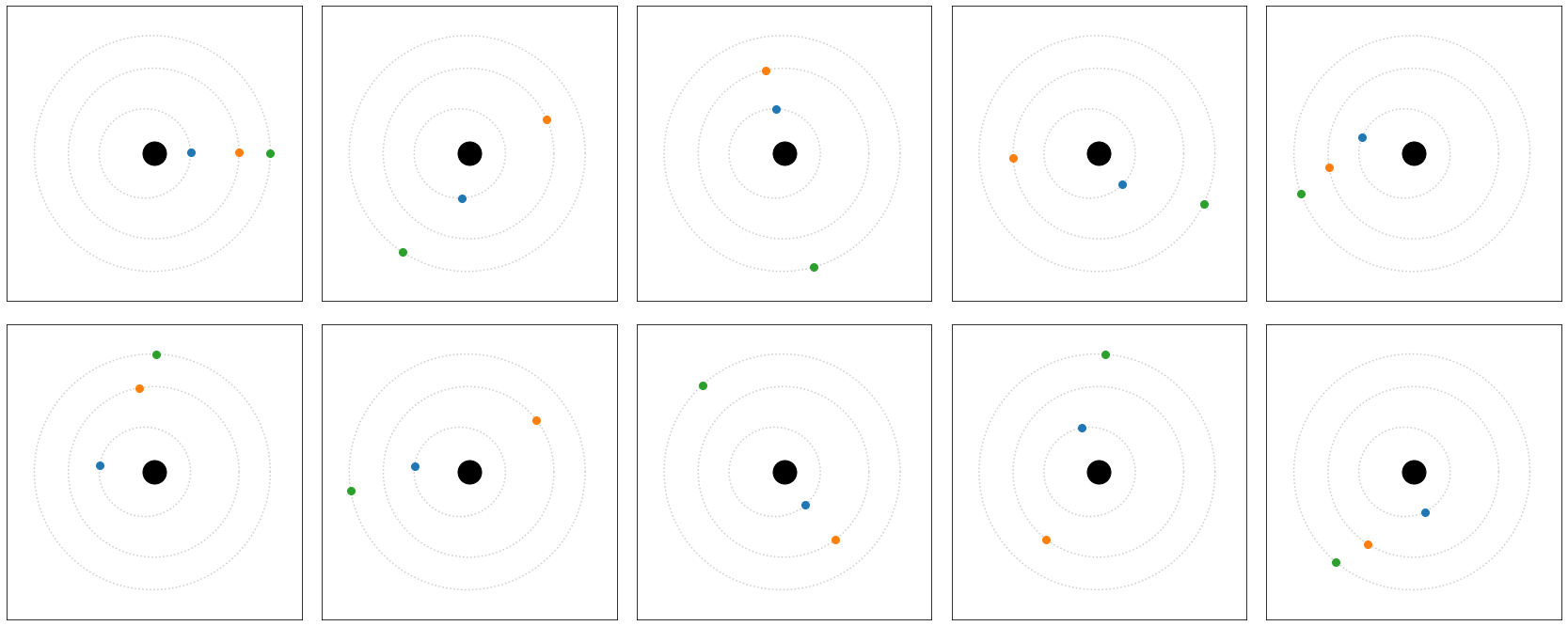
Given the fact that the actual periods of Earth, Venus and Mercury are not simple rational fractions of each other, I expect that this dance of alignments will continue to produce new arrangements for ever in reality, which is an exciting idea to me.

Retrograde

I was also curious to investigate the retrograde phenomenon, where planets appear to reverse direction when viewed against the ‘static’ backdrop of constellations. The problem becomes much easier now as the only part that matters is the ‘global’ direction one of the inner planets would be viewed as from Earth.

N = 1_000  # samples / year
T = 3.25  # years

t_r = np.linspace(0, T, int(T * N) + 1)
p_m = planet_v2(t_r, **MER)
p_v = planet_v2(t_r, **VEN)
p_e = planet_v2(t_r, **EAR)

v_me = p_m - p_e
v_ve = p_v - p_e

th_m = np.arctan2(*v_me.T)
th_v = np.arctan2(*v_ve.T)

And it’s relatively easy to calculate when either planet is in retrograde by checking if the derivative (or change from one timestep to the next) is going against the prevailing direction.

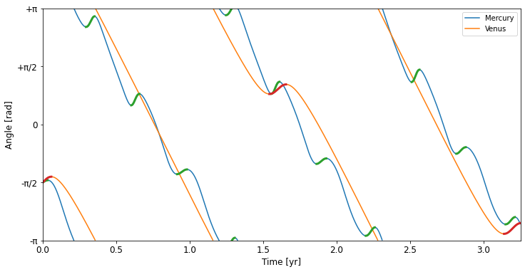
From this simple model, it looks like Mercury is in retrograde (shown in green) around 11x per 3.25 years (or 3.4/yr) and Venus (shown in red) around 2x / 3.25 years (or 0.6/yr). It is also interesting to see that both the relative position of Mercury and Venus against the stars, again ignoring inclination of planes, is somewhat similar but that is somewhat expected as both their orbits lay within Earth’s and I gave them all a similar starting point.

Looking at Wikipedia’s entries on expected moments of retrograde, it looks like this simplified model does a reasonable job at least at capturing the frequency of the event.

Conclusion

This was an interesting exploration and fun to learn more about the relative motion of our inner most planets. There are many ways I could have expanded on this work, e.g., by adding a third dimension to include each planet’s relative inclination from each other, etc., but for now this has satisfied my curiosity and I hope for anyone who has stumbled upon this page it has been an interesting read.

This page has converted from a Jupyter Notebook with most of the code removed for an improved reading experience, however, if you are interested in reading through the code and / or playing around with the original notebook, it can be downloaded here.